Spring Mass Damper System
Description of the problem
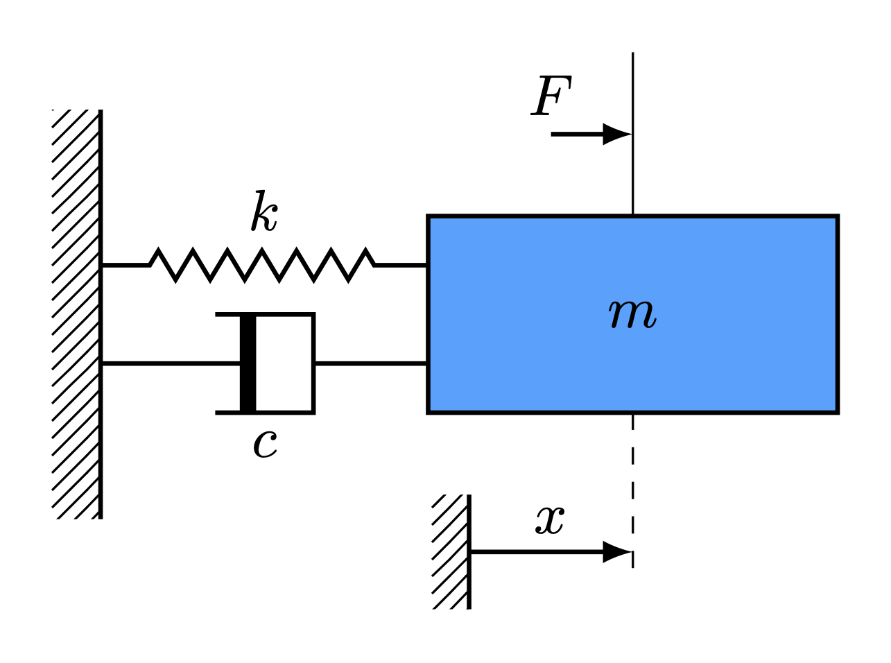
Consider the dynamics of a damped spring mass system governed by a second order differential equation given by
\begin{align} m\ddot{x}(t) + c\dot{x}(t) + k(t)x(t) = F(t) \end{align}
where \(m(t), c(t)\) and \(k(t)\) are the time-varying mass, damping and spring constants. Variable \(x(t)\) represents the displacement of the mass from the equilibrium and the external forcing is denoted by \(F(t)\). In a first-order state-space form with \(x_1 = x\) and \(x_2 = \dot{x}\), the continuous-time model (including its measurement equation) becomes
\begin{align} \dot{\boldsymbol{x}}(t) &= \begin{bmatrix} \dot{x}_1(t)\\ \dot{x}_2(t) \end{bmatrix} = \begin{bmatrix} 0 & 1\\ -\dfrac{k}{m} & -\dfrac{c}{m} \end{bmatrix} \begin{bmatrix} x_1(t)\\ x_2(t) \end{bmatrix} + \begin{bmatrix} 0 \\ 1 \end{bmatrix}F(t) = A_c\boldsymbol{x}(t) + B_cu(t),\\ \boldsymbol{y}(t) &= \begin{bmatrix} 1 & 0 \\ 0 & 1 \end{bmatrix}\begin{bmatrix} x_1(t)\\ x_2(t) \end{bmatrix} = C\boldsymbol{x}(t) + Du(t),\\ \end{align} where \begin{align} A_c = \begin{bmatrix} 0 & 1\\ -\dfrac{k}{m} & -\dfrac{c}{m} \end{bmatrix}, \quad B_c = \begin{bmatrix} 0 \\ 1 \end{bmatrix}, \quad C = \begin{bmatrix} 1 & 0 \\ 0 & 1 \end{bmatrix}, \quad D = \begin{bmatrix} 0 \\ 0 \end{bmatrix}. \end{align}
To compare with the identified models, analytical discrete-time models are generated by computing the state transition matrix (equivalent \(A_k\)) and the convolution integrals (equivalent \(B_k\) with a zero order hold assumption on the inputs). Because the system matrices are time varying, matrix differential equations are given by \begin{align} \dot{\Phi}(t, t_k) = A_c(t)\Phi(t, t_k), \quad \dot{\Psi}(t, t_k) = A_c(t)\Psi(t, t_k) + I, \end{align} \(\forall \ t \in [t_k, t_{k+1}]\), with initial conditions
\begin{align} \Phi(t_k, t_k) = \begin{bmatrix} 1 & 0\\ 0 & 1 \end{bmatrix}, \quad \Psi(t_k, t_k) = \begin{bmatrix} 0 & 0\\ 0 & 0 \end{bmatrix} \end{align} such that \begin{align} A_k = \Phi(t_{k+1}, t_k), \quad B_k = \Psi(t_{k+1}, t_k)B_c, \end{align} would represent the equivalent discrete-time varying system (true model). For the current investigation, the time variation profile of \begin{align} m(t) &= \exp(-0.1 * t),\\ c(t) &= 0.1 + 0.05\cos(t)\\ k(t) &= 1 + np.sin(2 * t^2). \end{align} The time interval of interest is 10 seconds, with the discretization sampling frequency set to be 10.
Given a time-history of \(\boldsymbol{x}(t_k)\) and \(u(t_k)\), the objective is to find a realization \((\hat{A}_k, \hat{B}_k, \hat{C}_k, \hat{D}_k)\) of the discrete-time linear model.
Code
The code below shows how to use the python systemID package to find a linear representation of the dynamics of the DC motor system.
First, import all necessary packages.
[1]:
import systemID as sysID

import numpy as np
import scipy.linalg as LA
from scipy.integrate import odeint

import matplotlib.pyplot as plt
from matplotlib import rc
plt.rcParams.update({"text.usetex": True, "font.family": "sans-serif", "font.serif": ["Computer Modern Roman"]})
rc('text', usetex=True)
plt.rcParams['text.latex.preamble'] = r"\usepackage{amsmath}"
[2]:
def m(t):
    return np.exp(-0.1 * t)
def c(t):
    return 0.1 + 0.05 * np.cos(t)
def k(t):
    return 1 + np.sin(2 * t**2)

state_dimension = 2
input_dimension = 1
output_dimension = 2

frequency = 10
dt = 1/frequency
[3]:
def Ac(t):
    return np.array([[0, 1], [-k(t)/m(t), -c(t)/m(t)]])

def dPhi(Phi, t):
    return np.matmul(Ac(t), Phi.reshape(state_dimension, state_dimension)).reshape(state_dimension ** 2)

def A(tk):
    A = odeint(dPhi, np.eye(state_dimension).reshape(state_dimension ** 2), np.array([tk, tk + dt]), rtol=1e-13, atol=1e-13)
    return A[-1, :].reshape(state_dimension, state_dimension)

def Bc(t):
    return np.array([[0], [1]])

def dPsi(Psi, t):
    return np.matmul(Ac(t), Psi.reshape(state_dimension, state_dimension)).reshape(state_dimension ** 2) + np.eye(state_dimension).reshape(state_dimension ** 2)

def B(tk):
    B = odeint(dPsi, np.zeros([state_dimension, state_dimension]).reshape(state_dimension ** 2), np.array([tk, tk + dt]), rtol=1e-13, atol=1e-13)
    return np.matmul(B[-1, :].reshape(state_dimension, state_dimension), Bc(tk))

def C(tk):
    return np.eye(state_dimension)

def D(tk):
    return np.zeros([output_dimension, input_dimension])

x0 = np.zeros(state_dimension)
true_system = sysID.discrete_linear_model(frequency, x0, A, B=B, C=C, D=D)
[4]:
number_experiments = 20
total_time_training = 10
number_steps_training = int(total_time_training * frequency + 1)

forced_inputs_training = []
forced_outputs_training = []
for i in range(number_experiments):
    forced_input_training = sysID.discrete_signal(frequency=frequency, data=np.random.randn(number_steps_training))
    forced_output_training = sysID.propagate(forced_input_training, true_system)[0]
    forced_inputs_training.append(forced_input_training)
    forced_outputs_training.append(forced_output_training)

free_outputs_training = []
free_x0_training = np.random.randn(state_dimension, number_experiments)
for i in range(number_experiments):
    model_free_response = sysID.discrete_linear_model(frequency, free_x0_training[:, i], A, B=B, C=C, D=D)
    free_output_training = sysID.propagate(sysID.discrete_signal(frequency=frequency, data=np.zeros([input_dimension, number_steps_training])), model_free_response)[0]
    free_outputs_training.append(free_output_training)
[5]:
tvokid_ = sysID.tvokid(forced_inputs_training, forced_outputs_training, observer_order=10, number_of_parameters=50)
p = 10
q = p
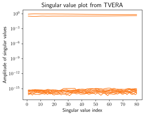
tvera_ = sysID.tvera(tvokid_.hki, tvokid_.D, free_outputs_training, state_dimension, p, q, apply_transformation=True)
concatenated_singular_values = np.concatenate([arr[np.newaxis, 0:10] for arr in tvera_.Sigma[:-p]], axis=0).T
fig = plt.figure(num=1, figsize=[5, 4])
ax = fig.add_subplot(1, 1, 1)
for i in range(concatenated_singular_values.shape[0]):
ax.semilogy(np.linspace(1, concatenated_singular_values.shape[1], concatenated_singular_values.shape[1]), concatenated_singular_values[i, :], color=(253/255, 127/255, 35/255))
plt.ylabel(r'Amplitude of singular values', fontsize=12)
plt.xlabel(r'Singular value index', fontsize=12)
plt.title(r'Singular value plot from TVERA', fontsize=15)
plt.xticks(fontsize=12)
plt.yticks(fontsize=12)
plt.tight_layout()
plt.show()
x0_id = np.zeros(state_dimension)
identified_system = sysID.discrete_linear_model(frequency, x0_id, tvera_.A, B=tvera_.B, C=tvera_.C, D=tvera_.D)
[6]:
total_time_testing = 10 - (p+1) * dt
number_steps_testing = int(total_time_testing * frequency + 1)
tspan_testing = np.linspace(0, total_time_testing, number_steps_testing)

input_testing = sysID.discrete_signal(frequency=frequency, data=np.sin(3 * tspan_testing))
output_testing_true = sysID.propagate(input_testing, true_system)[0]
output_testing_identified = sysID.propagate(input_testing, identified_system)[0]
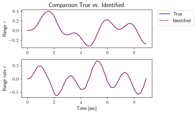
[7]:
fig = plt.figure(num=2, figsize=[7, 4])
ax = fig.add_subplot(2, 1, 1)
ax.plot(tspan_testing, output_testing_true.data[0, :], color=(11/255, 36/255, 251/255), label=r'True')
ax.plot(tspan_testing, output_testing_identified.data[0, :], '--', color=(221/255, 10/255, 22/255), label=r'Identified')
plt.ylabel(r'Range $r$', fontsize=12)
plt.title(r'Comparison True vs. Identified', fontsize=15)
ax.legend(loc='upper center', bbox_to_anchor=(1.18, 1.05), ncol=1, fontsize=12)
plt.xticks(fontsize=12)
plt.yticks(fontsize=12)
ax = fig.add_subplot(2, 1, 2)
ax.plot(tspan_testing, output_testing_true.data[1, :], color=(11/255, 36/255, 251/255))
ax.plot(tspan_testing, output_testing_identified.data[1, :], '--', color=(221/255, 10/255, 22/255))
plt.xlabel(r'Time [sec]', fontsize=12)
plt.ylabel(r'Range rate $\dot{r}$', fontsize=12)
plt.xticks(fontsize=12)
plt.yticks(fontsize=12)
plt.tight_layout()
plt.show()
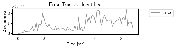
fig = plt.figure(num=3, figsize=[7, 2])
ax = fig.add_subplot(1, 1, 1)
ax.plot(tspan_testing, LA.norm(output_testing_true.data - output_testing_identified.data, axis=0), color=(145/255, 145/255, 145/255), label=r'Error')
plt.ylabel(r'2-norm error', fontsize=12)
plt.xlabel(r'Time [sec]', fontsize=12)
plt.title(r'Error True vs. Identified', fontsize=15)
ax.legend(loc='upper center', bbox_to_anchor=(1.18, 1.05), ncol=1, fontsize=12)
plt.xticks(fontsize=12)
plt.yticks(fontsize=12)
plt.tight_layout()
plt.show()
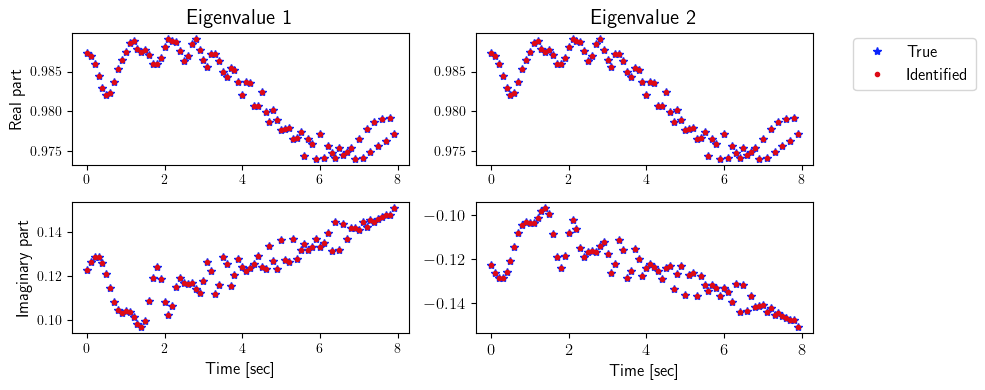
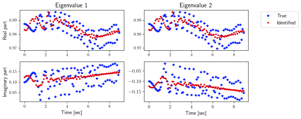
[8]:
ev_true = np.zeros([2, state_dimension, number_steps_testing])
ev_identified = np.zeros([2, state_dimension, number_steps_testing])
for i in range(number_steps_testing):
    for j in range(state_dimension):
        ev_true[0, j, i] = np.real(LA.eig(true_system.A(i * dt))[0])[j]
        ev_true[1, j, i] = np.imag(LA.eig(true_system.A(i * dt))[0])[j]
        ev_identified[0, j, i] = np.real(LA.eig(identified_system.A(i * dt))[0])[j]
        ev_identified[1, j, i] = np.imag(LA.eig(identified_system.A(i * dt))[0])[j]

fig = plt.figure(num=4, figsize=[10, 4])

ax = fig.add_subplot(2, 2, 1)
ax.plot(tspan_testing, ev_true[0, 0, :], '*', color=(11/255, 36/255, 251/255), label=r'True')
ax.plot(tspan_testing, ev_identified[0, 0, :], '.', color=(221/255, 10/255, 22/255), label=r'Identified')
plt.ylabel(r'Real part', fontsize=12)
plt.title(r'Eigenvalue 1', fontsize=15)

ax = fig.add_subplot(2, 2, 2)
ax.plot(tspan_testing, ev_true[0, 1, :], '*', color=(11/255, 36/255, 251/255), label=r'True')
ax.plot(tspan_testing, ev_identified[0, 1, :], '.', color=(221/255, 10/255, 22/255), label=r'Identified')
plt.title(r'Eigenvalue 2', fontsize=15)
ax.legend(loc='upper center', bbox_to_anchor=(1.3, 1.02), ncol=1, fontsize=12)

ax = fig.add_subplot(2, 2, 3)
ax.plot(tspan_testing, ev_true[1, 0, :], '*', color=(11/255, 36/255, 251/255), label=r'True')
ax.plot(tspan_testing, ev_identified[1, 0, :], '.', color=(221/255, 10/255, 22/255), label=r'Identified')
plt.ylabel(r'Imaginary part', fontsize=12)
plt.xlabel(r'Time [sec]', fontsize=12)

ax = fig.add_subplot(2, 2, 4)
ax.plot(tspan_testing, ev_true[1, 1, :], '*', color=(11/255, 36/255, 251/255), label=r'True')
ax.plot(tspan_testing, ev_identified[1, 1, :], '.', color=(221/255, 10/255, 22/255), label=r'Identified')
plt.xlabel(r'Time [sec]', fontsize=12)

plt.xticks(fontsize=12)
plt.yticks(fontsize=12)

plt.tight_layout()
plt.show()
[9]:
ev_true = np.zeros([2, state_dimension, number_steps_testing - p])
ev_identified = np.zeros([2, state_dimension, number_steps_testing - p])
for i in range(number_steps_testing - p):
    for j in range(state_dimension):
        O1_true = sysID.observability_matrix(true_system.A, true_system.C, p, tk=i * dt, dt=dt)
        O2_true = sysID.observability_matrix(true_system.A, true_system.C, p, tk=(i + 1) * dt, dt=dt)
        ev_true[0, j, i] = np.real(LA.eig(np.matmul(LA.pinv(O1_true), np.matmul(O2_true, true_system.A(i * dt))))[0])[j]
        ev_true[1, j, i] = np.imag(LA.eig(np.matmul(LA.pinv(O1_true), np.matmul(O2_true, true_system.A(i * dt))))[0])[j]

        O1_identified = sysID.observability_matrix(identified_system.A, identified_system.C, p, tk=i * dt, dt=dt)
        O2_identified = sysID.observability_matrix(identified_system.A, identified_system.C, p, tk=(i + 1) * dt, dt=dt)
        ev_identified[0, j, i] = np.real(LA.eig(np.matmul(LA.pinv(O1_identified), np.matmul(O2_identified, identified_system.A(i * dt))))[0])[j]
        ev_identified[1, j, i] = np.imag(LA.eig(np.matmul(LA.pinv(O1_identified), np.matmul(O2_identified, identified_system.A(i * dt))))[0])[j]

fig = plt.figure(num=4, figsize=[10, 4])

ax = fig.add_subplot(2, 2, 1)
ax.plot(tspan_testing[:-p], ev_true[0, 0, :], '*', color=(11/255, 36/255, 251/255), label=r'True')
ax.plot(tspan_testing[:-p], ev_identified[0, 0, :], '.', color=(221/255, 10/255, 22/255), label=r'Identified')
plt.ylabel(r'Real part', fontsize=12)
plt.title(r'Eigenvalue 1', fontsize=15)

ax = fig.add_subplot(2, 2, 2)
ax.plot(tspan_testing[:-p], ev_true[0, 1, :], '*', color=(11/255, 36/255, 251/255), label=r'True')
ax.plot(tspan_testing[:-p], ev_identified[0, 1, :], '.', color=(221/255, 10/255, 22/255), label=r'Identified')
plt.title(r'Eigenvalue 2', fontsize=15)
ax.legend(loc='upper center', bbox_to_anchor=(1.3, 1.02), ncol=1, fontsize=12)

ax = fig.add_subplot(2, 2, 3)
ax.plot(tspan_testing[:-p], ev_true[1, 0, :], '*', color=(11/255, 36/255, 251/255), label=r'True')
ax.plot(tspan_testing[:-p], ev_identified[1, 0, :], '.', color=(221/255, 10/255, 22/255), label=r'Identified')
plt.ylabel(r'Imaginary part', fontsize=12)
plt.xlabel(r'Time [sec]', fontsize=12)

ax = fig.add_subplot(2, 2, 4)
ax.plot(tspan_testing[:-p], ev_true[1, 1, :], '*', color=(11/255, 36/255, 251/255), label=r'True')
ax.plot(tspan_testing[:-p], ev_identified[1, 1, :], '.', color=(221/255, 10/255, 22/255), label=r'Identified')
plt.xlabel(r'Time [sec]', fontsize=12)

plt.xticks(fontsize=12)
plt.yticks(fontsize=12)

plt.tight_layout()
plt.show()