DC Motor System
Description of the problem
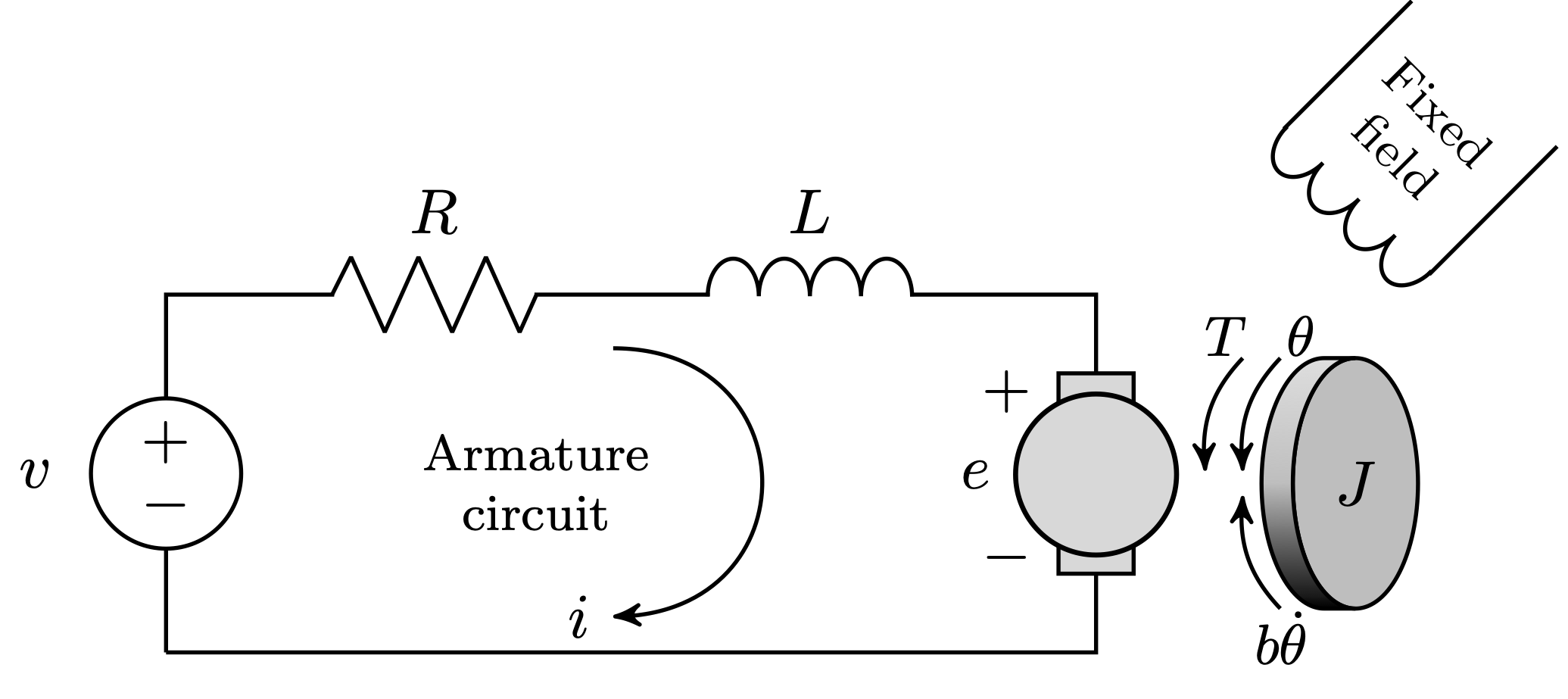
The DC motor is a frequently used actuator that delivers immediate rotational movement. By pairing it with components such as wheels, drums, or cables, it can also generate linear motion. The input of the system is the voltage source (\(V\)) applied to the motor’s armature, while the output is the position of the shaft (\(\theta\)). The rotor and shaft are assumed to be rigid. We further assume a viscous friction model, that is, the friction torque is proportional to shaft angular velocity.
The differential equations, in state-space form, by choosing the motor position \(x_1=\theta\), motor speed \(x_2 = \dot{\theta}\) and armature current \(x_3=i\) as the state variables, are
\begin{align} \dot{\boldsymbol{x}}(t) &= \begin{bmatrix} \dot{x}_1(t)\\ \dot{x}_2(t)\\ \dot{x}_3(t) \end{bmatrix} = \begin{bmatrix} 0 & 1 & 0\\ 0 & -\dfrac{b}{J} & \dfrac{K}{J}\\ 0 & -\dfrac{K}{L} & -\dfrac{R}{L} \end{bmatrix} \begin{bmatrix} x_1(t)\\ x_2(t)\\ x_3(t) \end{bmatrix} + \begin{bmatrix} 0 \\ 0\\ \dfrac{1}{L} \end{bmatrix}V(t) = A_c\boldsymbol{x}(t) + B_cu(t),\\ \boldsymbol{y}(t) &= \begin{bmatrix} 0 & 0 & 1 \end{bmatrix}\begin{bmatrix} x_1(t)\\ x_2(t)\\ x_3(t) \end{bmatrix} = C\boldsymbol{x}(t) + Du(t),\\ \end{align} where \begin{align} A_c = \begin{bmatrix} 0 & 1 & 0\\ 0 & -\dfrac{b}{J} & \dfrac{K}{J}\\ 0 & -\dfrac{K}{L} & -\dfrac{R}{L} \end{bmatrix}, \quad B_c = \begin{bmatrix} 0 \\ 0\\ \dfrac{1}{L} \end{bmatrix}, \quad C = \begin{bmatrix} 0 & 0 & 1 \end{bmatrix}, \quad D = \begin{bmatrix} 0 \\ 0 \end{bmatrix}. \end{align} Assuming that \(u(\tau)\) is constant between sample times, i.e. \(u(\tau) = u(k\Delta t)\) for \(k\Delta t\leq \tau < (k+1)\Delta t\), let’s define the discrete-time model \begin{align} \boldsymbol{x}_{k+1} &= A\boldsymbol{x}_{k} + Bu_k,\\ \boldsymbol{y}_{k} &= C\boldsymbol{x}_{k} + Du_k, \end{align} where \begin{align} A = e^{A_c\Delta t}, \quad B_c = \int_{0}^{\Delta t}e^{A_ct}\mathrm{d}tB_c. \end{align} Given a time-history of \(\boldsymbol{x}(t_k)\) and \(u(t_k)\), the objective is to find a realization \((\hat{A}, \hat{B}, \hat{C}, \hat{D})\) of the discrete-time linear model.
Code
The code below shows how to use the python systemID package to find a linear representation of the dynamics of the DC motor system.
First, import all necessary packages.
[1]:
import systemID as sysID

import numpy as np
import scipy.linalg as LA

import matplotlib.pyplot as plt
from matplotlib import rc
plt.rcParams.update({"text.usetex": True, "font.family": "sans-serif", "font.serif": ["Computer Modern Roman"]})
rc('text', usetex=True)
plt.rcParams['text.latex.preamble'] = r"\usepackage{amsmath}"
[2]:
J = 3.2284e-6
b = 3.5077e-6
K = 0.0274
R = 4
L = 2.75e-6

state_dimension = 3
input_dimension = 1
output_dimension = 1

frequency = 10
dt = 1/frequency
[3]:
Ac = np.array([[0, 1, 0], [0, -b/J, K/J], [0, -K/L, -R/L]])
Bc = np.array([[0], [0], [1/L]])

(Ad, Bd) = sysID.continuous_to_discrete_matrices(dt, Ac, Bc=Bc, expansion=True)

def A(t):
    return Ad
def B(t):
    return Bd
def C(t):
    return np.array([[1, 0, 0]])
def D(t):
    return np.zeros([output_dimension, input_dimension])

x0 = np.zeros(state_dimension)
true_system = sysID.discrete_linear_model(frequency, x0, A, B=B, C=C, D=D)
[4]:
total_time_training = 5
number_steps_training = int(total_time_training * frequency + 1)

input_training = sysID.discrete_signal(frequency=frequency, data=np.random.randn(number_steps_training))
output_training = sysID.propagate(input_training, true_system)[0]
[5]:
okid_ = sysID.okid_with_observer([input_training], [output_training], observer_order=10, number_of_parameters=50)
p = 20
q = p
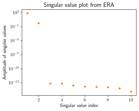
era_ = sysID.era(okid_.markov_parameters, state_dimension=state_dimension, p=p, q=q)
fig = plt.figure(num=1, figsize=[5, 4])
ax = fig.add_subplot(1, 1, 1)
ax.semilogy(np.linspace(1, 10, 10), np.diag(era_.Sigma)[0:10], '*', color=(253/255, 127/255, 35/255))
plt.ylabel(r'Amplitude of singular values', fontsize=12)
plt.xlabel(r'Singular value index', fontsize=12)
plt.title(r'Singular value plot from ERA', fontsize=15)
plt.xticks(fontsize=12)
plt.yticks(fontsize=12)
plt.tight_layout()
plt.show()
x0_id = np.zeros(state_dimension)
identified_system = sysID.discrete_linear_model(frequency, x0_id, era_.A, B=era_.B, C=era_.C, D=era_.D)
Error OKID = 2.183526586242027e-13
[6]:
total_time_testing = 20
number_steps_testing = int(total_time_testing * frequency + 1)
tspan_testing = np.linspace(0, total_time_testing, number_steps_testing)

input_testing = sysID.discrete_signal(frequency=frequency, data=np.sin(3 * tspan_testing))
output_testing_true = sysID.propagate(input_testing, true_system)[0]
output_testing_identified = sysID.propagate(input_testing, identified_system)[0]
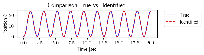
[7]:
fig = plt.figure(num=2, figsize=[7, 3])
ax = fig.add_subplot(2, 1, 1)
ax.plot(tspan_testing, output_testing_true.data[0, :], color=(11/255, 36/255, 251/255), label=r'True')
ax.plot(tspan_testing, output_testing_identified.data[0, :], '--', color=(221/255, 10/255, 22/255), label=r'Identified')
plt.ylabel(r'Position $\theta$', fontsize=12)
plt.xlabel(r'Time [sec]', fontsize=12)
plt.title(r'Comparison True vs. Identified', fontsize=15)
ax.legend(loc='upper center', bbox_to_anchor=(1.18, 1.05), ncol=1, fontsize=12)
plt.xticks(fontsize=12)
plt.yticks(fontsize=12)
plt.tight_layout()
plt.show()
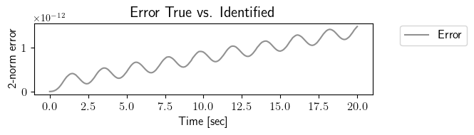
fig = plt.figure(num=3, figsize=[7, 2])
ax = fig.add_subplot(1, 1, 1)
ax.plot(tspan_testing, LA.norm(output_testing_true.data - output_testing_identified.data, axis=0), color=(145/255, 145/255, 145/255), label=r'Error')
plt.ylabel(r'2-norm error', fontsize=12)
plt.xlabel(r'Time [sec]', fontsize=12)
plt.title(r'Error True vs. Identified', fontsize=15)
ax.legend(loc='upper center', bbox_to_anchor=(1.18, 1.05), ncol=1, fontsize=12)
plt.xticks(fontsize=12)
plt.yticks(fontsize=12)
plt.tight_layout()
plt.show()
[8]:
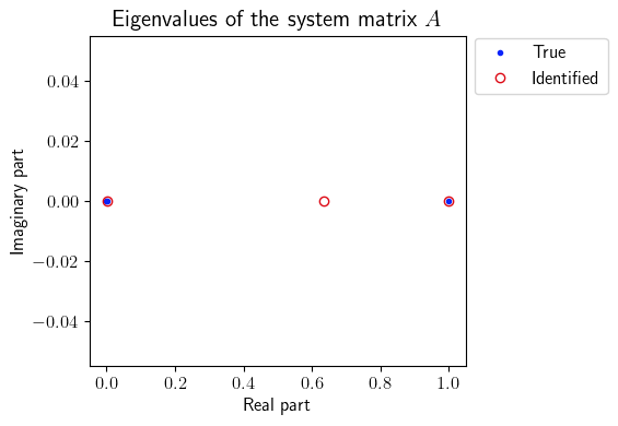
ev_true = LA.eig(A(0))[0]
ev_identified = LA.eig(era_.A(0))[0]
print('True eigenvalues:', ev_true)
print('Identified eigenvalues:', ev_identified)

fig = plt.figure(num=4, figsize=[6, 4])

ax = fig.add_subplot(1, 1, 1)
ax.plot(np.real(ev_true), np.imag(ev_true), '.', color=(11/255, 36/255, 251/255), label=r'True')
ax.plot(np.real(ev_identified), np.imag(ev_identified), 'o', mfc='none', color=(221/255, 10/255, 22/255), label=r'Identified')
plt.ylabel(r'Imaginary part', fontsize=12)
plt.xlabel(r'Real part', fontsize=12)
plt.title(r'Eigenvalues of the system matrix $A$', fontsize=15)
ax.legend(loc='upper center', bbox_to_anchor=(1.2, 1.02), ncol=1, fontsize=12)
plt.xticks(fontsize=12)
plt.yticks(fontsize=12)

plt.tight_layout()
plt.show()
True eigenvalues: [1.00000000e+00+0.j 2.67821742e-03+0.j 1.32348898e-23+0.j]
Identified eigenvalues: [1.        +0.j 0.00267822+0.j 0.63406493+0.j]